Transmission lines are dual conductor (often twin wire) lines that act as transverse electromagnetic mode (TEM) wave guides for electromagnetic waves. These are the simplest structures that guide waves and they have much in common with microwave waveguides (hollow rectangular or circular pipes that transmit EM waves), surface wave devices which guide waves glued to their surfaces (eg HF surface waves on the sea) and optical fibres. They are also the ONLY way of transporting signals in radiofrequency circuits. Single wire transport is not encouraged!

Our picture of a transmission line is the simple twin wire line as follows.

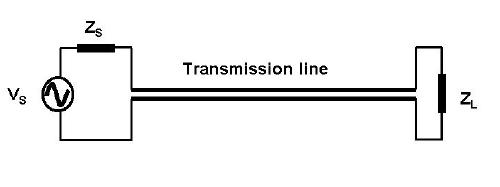
This simple schematic is all there is to a practicable and useful transmission line. The other type of most interest is the coaxial line where one of the wires is a pipe that surrounds the centre conductor.

Examples of transmission lines include the ribbon cable used for VHF television or the RG-58 coax (pronounced CO-AX and short for coaxial cable) that we use most often in the lab. You can make a simple twin wire line yourself by carefully twisting two thin wires together (twisted pair). Another example is a so called "strip line" in which a copper track is etched onto a two sided circuit board above a ground plane. The crucial design issues with transmission lines are that the forward and the return current carrying wires are close together having large mutual coupling and that the characteristics of the line do not vary along its length

One obvious advantage of coax over the twin wire line is that the return current in the pipe (the outer conductor or braid on flexible coax like RG-58) flows on the inside surface and not on the outside surface. Due to the skin effect, the signal carried on the line is not radiated into the environment outside the cable. Conversely radiofrequency noise in the environment cannot enter the cable either. It induces RF currents on the outside of the braid. Coaxial cable minimises RFI (radiofrequency interference) arising from the signals it carries and minimises the effect of external RFI on these signals.

THE TELEGRAPHIST EQUATIONS

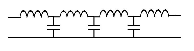
The telegraphist equations relate to the distributed impedance or lumped picture of a transmission line. The distributed picture of a transmission line is shown in the following figure. The inductor symbols are the L, inductance per unit length and the capacitor symbols are C, capacitance per unit length. Obviously it looks like a filter. There is an important difference though in that this circuit approximates a filter which does not distort or attenuate amplitude and produces a phase shift which is linear in the frequency and the number of line sections. Moreover it does so for any value of L or C as long as these are infinitesimal in size and therefore infinite in number and constant in value. Consider the following diagram:

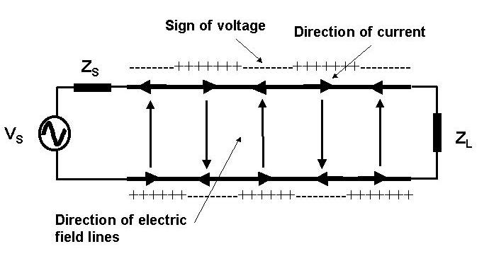
For an infinitely long transmission line, the current that propagates with the voltage wave points in the direction of propagation of the wave on the wire where the voltage is instantaneously positive (see the figure below for a wave propagating to the right).

The basic physics of the transmission line is relatively simple (see reference (2)). The voltage and current propagating along the line satisfy the Telegraphist equations

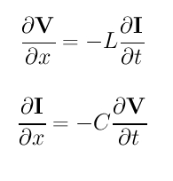
where x is the distance along the line, t is the time, L is the inductance per unit length of the line and C is the capacitance per unit length. By voltage we mean the potential difference between the two wires in the cross-section perpendicular to the wires. The current is equal and opposite in each wire. If we are talking about coax we mean the voltage between the centre conductor and earth and the equal and opposite current in each. Remember in our discussion about inductance that one non-ideal effect was distributed capacitance along the inductance coil which causes a wave to propagate along the coil. Transmission lines behave in a similar way. A transmission line has distributed C and L per unit length along the line. In combination these produce wave motions of voltage and current along the line.

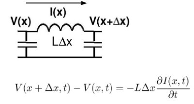
It is relatively easy to derive the telegraphist equations. Consider the following figures where L and C refer to the inductance and capacitance per unit length of a distributed transmission line. Each circuit is displaced slightly along the direction x of the line. Both I and V are also functions of time. We assume that the line segment is short enough that we can apply Kirchoff's current and voltage laws individually to each segment.

Applying Kirchoff's voltage law shows that the change in voltage along the line is given by the inductive voltage drop of the varying current.

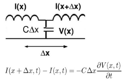
Applying Kirchoff's current law to the node at the capacitor shows that the change in current along the line is given by the current lost in the capacitance.

These equations are exactly the Telegraphist's equations as stated above. What is interesting is that we could eliminate I between the two telegraphist equations to derive a single wave equation for the voltage V along the line:

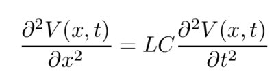
This should be compared to the wave equation for electromagnetic waves derived in the chapter on electromagnetism. The wave equation describes the propagation of a voltage disturbance along the line. A similar equation can also be deriveed for the current, I. When excited by a sinusoidal function generator, the line supports a sinusoidal wave that propagates along the line from the source to the load. This forward wave (let us say, travelling toward positive x from the source at the left) is described by V = V_F exp(jkx) where k = &omega /v is the wavenumber, &omega is the radian frequency of the wave and v the phase velocity of the line. The phase velocity is given by v = 1/(LC)^1/2. The wave number is related to the wavelength (of the sine wave) by &lambda = 2 &pi /k. It is a trivial matter to show that this sinusoidal wave satisfies the wave equation and Telegraphist equations. In addition to this forward wave there may also be a reverse wave satisfying V = V_B exp(-jkx). This corresponds to a wave that propagates in the reverse direction to the forward wave. A reverese wave can arise when wave energy in the forward wave is reflected at the end of the line. It could also arise of course if there is a signal source located at the right hand end of the line. This wave also satisfies the wave equation Telegraphist equations.

By substituting these equations for the forward and reverse wave into the Telegraphist equations you can obtain expressions for the relevant forward and reverse currents I in each case. Remember that for each voltage wave there is a corresponding current wave and that the current wave is in phase with the voltage wave

If you are having trouble visualising this have a look at the JAVA applets of transmssion line waves for various values of the terminating impedance shown below.

It can also be shown from the Telegraphist equations that the ratio of the voltage to current in the travelling wave is given by V/I = Z₀ where Z₀ = (L/C)^1/2. The quantity Z₀ is the characteristic impedance of the line. Thus for example, the TV ribbon cable used in VHF TV is a twin wire transmission line of characteristic impedance 300 &Omega and RG-58 is unbalanced coaxial cable of characteristic impedance 50 &Omega. For loss free lines, the characteristic impedance is real. This is an amazing fact about transmission lines. Where did all those L and C reactances go to? Remember the discussions about hook-up wiring at RF?. Now we know how to cable our signals all around the place.

In future, use a transmission line and not hook-up wires! Of course when using print circuit boards to make radiofrequency circuits you must use the tracks on the board as strip transmission lines or strip lines, where the track itself is the active transmission line wire, the PCB dielectric is the transmission line dielectric and the earth plane under the board is the return path.

The real value of Z₀ does not even imply that power is dissipated as heat. It simply states that the voltage and current are in phase and power is lost by propagation instead of dissipation. The wave propagates away and never comes back. After all, having something fly away is just as effective a means of losing it as destroying it.

The reverse wave (if there is one) would, by symmetry, have the current pointing in the opposite direction. This is interesting because it means that it should be possible to separate out the forward and the reverse wave in order to resolve the so called forward power P_F = V_F²/Z₀ amd the reverse power P_R = V_R²/Z₀

What would happen if Z_L = Z₀? Clearly the wave would pass into Z_L and vanish by heat dissipation in Z_L. Thus terminating the line in Z₀ fools the wave into thinking that the line is infinitely long.

What happens if Z_L and Z₀ are different? This is in fact how one produces the reflected wave in the first place; by not correctly terminating the line. This is usually to be avoided. Moreover one would end up with a bit of a mess if Z_S is not equal to Z₀ either.

Ex 12. Given the above description of how waves propagate along a transmission line, can you suggest a way of measuring individually the forward and the reflected voltage wave amplitudes on a transmission line?

Using the same technique one can show that the four port relations of a transmission line are given by the following equations,

Where the subscript i refers to the voltage and current toward the generator and the subscript o refers to the voltage and current toward the load. l is the length of the line.

Often instrumentation which measures reflected power and reflection coefficient provides the output in the form of the Voltage Standing Wave Ratio (VSWR or SWR). VSWR is the ratio of the maximum voltage amplitude along a line to the minimum value. For a matched line VSWR = 1. It may be derived from the reflection coefficient as follows.

From this we note that a transmission line can be employed to transform impedance. The quantity kl is the propagation constant or wavevector and is is given by 2&pi l/&lambda where l/&lambda is the electrical length of the line.

Transmission lines can be lossy. Lossiness (a word from RF land) arises by internal resistance in the conductors used to make the line, losses due to finite conductance in the dielectric or radiation from the line. Lossiness is described mathematically by a complex value of the propagation constant, k.

The following JAVA applets show the transmission line waves of voltage (green) and current (red) as a function of distance along a line of length 1.5 wavelengths. The voltage is measured directly across the line. The direction of positive current flow is measured on the line where the voltage is positive. It always points in the direction of travel of the wave. The source is at the left end (x = 0) and the load is at the right end (here x = 1.5). The source impedance is 50&Omega so that the reflected wave is not reflected again at the source. Thus the input impedance of the line divides down the Thevenin source voltage of 1 volt. The voltages are in Volts and the current in Amperes.

Note that the electrical length of the lines in each case is 1.5 wavelengths. According to the impedance formula, the load impedance is transformed into itself at the front of the line. IE the input impedance at the source end is equal to the load impedance. This is obviously a special case. Because the source end is terminated however, the behaviour of shorter lines for the same source Thevenin equivalent, is the same. For example the voltage and current waveforms along a line of length 0.25 wavelengths are those shown between x = 1.25 and 1.5 wavelengths near the end of the line.

Ex. 15 Model the following lumped LC transmission line circuit in MATLAB for a terminating resistance of 50&Omega . (a) Plot the voltage and the current amplitudes along the line from the source to termination. (b) Plot the phase of the voltage and currents along the line. (c) Describe in words what is happening. In a real transmission line the inductance and capacitance values are zero whilst the inductance and capacitance per unit length are finite. So be sure to investigate smaller and smaller L's and C's in your model. Include plots in your log book.

Ex. 16. Take a long RG58 coaxial cable. Set up the FSH-3 spectrum analyser for transmission measurement. Measure the insertion loss from 1 MHz - 3GHz. Document your measurements.

Ex. 17. Using the FSH-3 analyser and a ~ 0.20 m length of coaxial cable terminated in an open circuit, connect the tracking generator output to the input of the analyser and Tee the cable at the input

(i) Locate the frequencies where the impedance at the coaxial cable at its input goes through zero and infinity (DC - 3 GHz).

(ii) How do you explain the results?

(iii) Compare the measured frequencies with the theoretical values. From this can you calculate the speed of propagation of electromagnetic waves in the cable?

Ex. 18. Repeat Ex. 17 for a short circuit terminated line. Do the zero and infinite impedances occur at the same frequencies? Can you explain the results?

Example. Using the four port transformation of a transmission line show that the line can approximate the following T-circuit, with the values

X/2 = Z_o tan(&omega l/2v) and B = (1/Z_o) sin(&omega l/v)



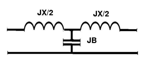
Moreover in the approximation that &omega l/v < &pi /4:

X = Z_o &omega l/v and B = &omega l/Z_o v.

Thus defining an inductance and capacitance of the element. We may therefore conclude that if the terminating impedance is lower than the characteristic impedance, then the short line looks like a series inductance and if the terminating impedance is greater than the characteristic impedance then the short line looks like a capacitor.

The above example shows the most common way of replacing inductors and capacitors with transmission lines in strip line filters