NETWORKS

Gerard Borg
ENGN4545
2007

Here we briefly look at some common ways to describe linear networks. Networks are referred to as linear if the components which comprise them have a linear relationship between voltage and current. An immediate consequence of this is that the variation of voltage between two nodes in the network with the current into those nodes must be linear (could it ever be quadratic?). It does not matter whether there are transistors and reactances or whatever in the network as long as we confine ourselves to a range of voltage and current oscillation amplitudes for which all components behave linearly. 1. THEVENIN AND NORTON EQUIVALENT CIRCUITS. For example consider the following linear blackbox with some wires hanging out... 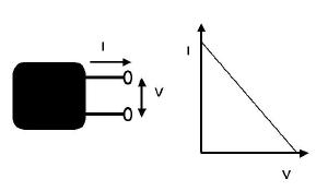If resistors of various values are connected across the output terminals, then the variation in the magnitude of the current versus voltage would look as on the graph at the right. Clearly, for all we care, the blackbox circuit really looks like the following, 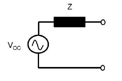This is the Thevenin (pronounced in between 'Tayvna' and 'Tevnang') equivalent of the black box network. It behaves as a voltage source of value equal to the open circuited voltage of the network and an output impedance equal to that obtained between the terminals with the internal voltage (and current) sources suppressed. An obvious variation is the Norton equivalent as follows, 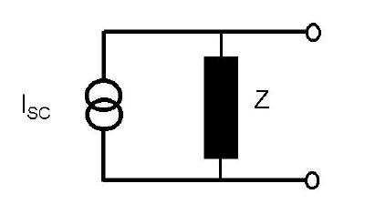Ex.8. Prove that maximum power is transferred from the source to the load when the output impedance is equal to the complex conjugate of the load impedance. The principle proven here is the principle of matching a source to a load. Thus we see that matching is a question of maximum power transfer to the load. A much bigger constraint on matching whenever a transmission line is involved is that the load and source impedances in question must also equal the characteristic impedance of the transmission line in order to avoid the reflection of radio frequency power back from the load to the source. Since the latter is usually about 50 - 300Ω s, in practice we try to match everything to this value. The impedance on which a particular device operates is an important parameter in the specification of an RF circuit. 2. S-PARAMETERS One method of characterising linear devices that permits practical measurements to be performed, are the S-parameters. 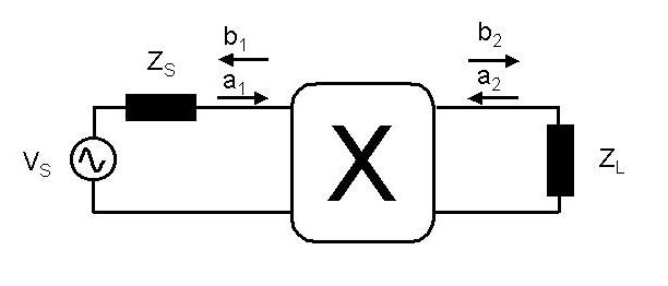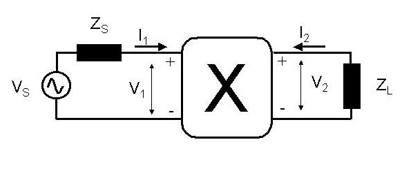These are easy to understand if you have already read about reflection of transmission line waves. The following shows the idea. Here I have drawn a four port device "X" under test. It is driven from a terminated source and feeds a load. In practice, this load does not have to be at the characteristic impedance of the system. For example, imagine that the device under test were a transistor coupling power to the load. The load would be chosen with an impedance equal to the complex conjugate of the output impedance of the transistor. The source sends a signal a1 toward X. In general we would measure a reflected signal b1 return from X. The rest of the signal a1 is transmitted by X and partly becomes b2 which propagates toward the load. The signal b1 arises partly because X is not terminated at its input and partly because the load ZL is not a proper termination. In the latter case a reflected signal a2 results which is then transferred back to the input of X and contributes to b1. Similarly part of a2 is reflected at the output and contributes to the rest of b2. The S-paramters are then defined by the following, b1 = S11a1 + S12a2 and, b2 = S21a1 + S22a2 S11 is the input reflection coefficient or "return loss", S12 is the reverse transmission coefficient, S21 is the forward transmission coefficient and S22 is the output reflection coefficient. The advantage of the S-parameters is the ease with which they can be measured since all measurements involve terminated lines. S11 = (b1/a1)|a2=0. VIZ let ZL = Z0 and measure the reflection coefficient. Thus S11 is the usual reflection coefficient. S21 = (b2/a1)|a2=0. VIZ let ZL = Z0 and measure the ratio of the transmitted to the incoming signal. Therefore, the insertion loss (gain) is S21 S22 = (b2/a2)|a1=0. VIZ swap the source and ZL, let ZL = Z0 and measure the reflection coefficient. S12 = (b1/a2)|a1=0. VIZ swap the source and ZL, let ZL = Z0 and measure the ratio of the transmitted to the incoming signal.

An alternative way to describe a four port network is in terms of the y-parameters. These are admittance parameters and will become useful when we try to analyse the performance of transistors. The figure shows the sense of the voltages and the currents used in their definition.

The y-parameters are given by.

where y_i is the short circuit input admittance, y_r the short circuit reverse-transfer admittance, y_f the short circuit forward-transfer admittance and y_o the short circuit output admittance.

For future reference, the y-parameters can be related to the S-parameters by the following formulae.

4. A TECHNIQUE FOR ANALYSING LINEAR CIRCUITS OF ARBITRARY COMPLEXITY

Using the S-parameters, one is equipped to do RF circuit designs based on transistor data sheets. However there is now a dilemma. Even the simplest common emitter amplifier presents an horrendous design project for a small signal transistor like the one shown above due to the quantity of algebra involved. Repeat this hundreds of times a year and before you know it, months have been squandered with pen and paper. One alternative, which in the nearer to longer term should be pursued, is to become acquainted with SPICE (Simulation Program with Integrated Circuit Emphasis) or PSPICE (the PC windows version). As the name suggests, SPICE has a large amount of support for specific transistors.

I now present a MATLAB program model that can be used to analyse a linear circuit with a single current (or voltage) source. We derive the model in order to treat specifically four port devices which have been characterised in terms of the y-parameters. However we will also look at the case of routine four port devices such as transformers and transmission lines. The obvious up-side is that it will free you from the algebra and may also teach you something about circuits. However you may also have a preference for some commercial or freeware package that does the job and you are free to use that instead if you wish.

The following node from a potentially vast circuit shows the idea. The labels j,k and l refer to arbitrary neghbouring nodes to node i. The node i is fed by a current I which most of the time will be zero. Note the directions of the currents and voltages.

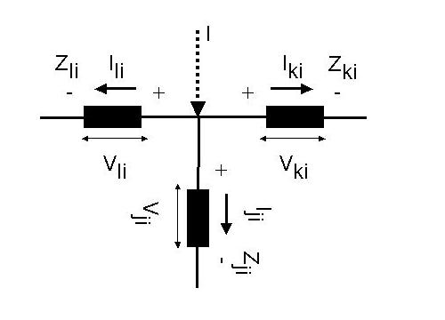
By applying Kirchhoff's current rule to this circuit we have,

The sign convention for voltage is V_ji = V_i - V_j. By summing up the currents into every node in the network we obtain the following set of equations.

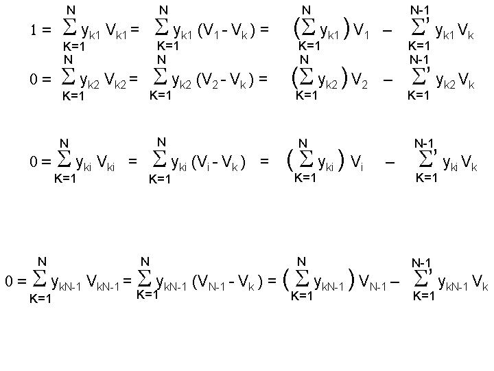
In this set, node 1 has the current source (1 Ampere) connected to it (all the others have nothing connected so they are zero), node N is ground and the ' on the summations means do not include the index i in this sum. Of course if let the corresponding y_ii = 0 then this amounts to the same thing. The other end of the current source is connected to ground. In the case of the first equation i = 1, the second equation, i = 2, the ith equation, i = i and the (N-1)th equation i = N-1. The voltage V_N = 0 as it is the voltage of ground with respect to ground and this explains why the last sums only go to N-1.

Thus in setting up the model parameters, remember that the current source always feeds into node 1 and that ground is connected at node N. From the above equations it should be clear that the y_Ni are required whereas the y_iN are not. All other y_ik for i,k < N must be provided (otherwise they are set to zero as is required for nodes that are not connected). These equations form an N-1 by N-1 matrix that can be inverted for the V_i's once we specify the y_ij's. The MATLAB program solve.m does this inversion and plots the results. You have to define a circuit node topology and specify the admittances.

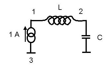
To calculate the y_ij's, let's consider a simple example; A series LC circuit fed by a current source. The MATLAB file can be found in program LC.m. The number of frequencies, Nvals, and the number of nodes, N = 3, as well as the y_ij's have to be specified.

To run the code put "LC" at the top in "solve.m" and run "solve" |ret> at the MATLAB command prompt. The parameter "inode" in the plotting lines of "solve.m" is the node at which the impedance is to be plotted (here inode = 1).

It is a simple matter to replace the current source by a voltage source. The model computes the voltage at all nodes in the network with respect to ground given a current source of 1 Ampere at node 1. To find the voltages at all nodes for a 1 Volt voltage source connected in place of the current source, divide all the other voltages in the network by V₁. It is clear that just about anything can be calculated for an arbitrarily vast network and it is a simple matter to rework the derivation to include current sources in more than one place. It is more important for us however to extend the model to include transistors, transformers and transmission lines.

4.1 Taking Care of Transistors

Given the y-parameters (which can be obtained from the S-parameters), one can easily include bipolar transistors into the above scheme. Take a look at the following four port representation of the transistor.

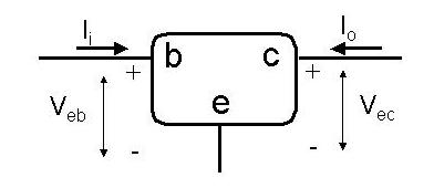
There are three current nodes connected at the terminals. In terms of the y-parameters we may write,

We need to rewrite these for each of the current nodes connected at b, e and c. Consider the base, b. The current I_i into the base can be rewritten,

where the voltages are from e,c to b, the base and follow our previous conventions. This means that the current into the base effectively flows to both the emitter and the collector as if there were simple impedances connected between them. Consider the collector, c. The current I_o into the collector can be rewritten,

For the emitter node we have to compute the current flowing into the emitter. This current is I_e = -(I_i + I_o). Finally,

4.2 Transformers

A transformer is simply a four port device as follows.

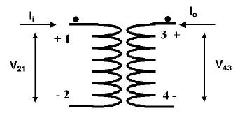
The basic equations of the transformer are,

where L₁ is the primary (1 - 2) inductance, L₂ is the secondary (3 - 4) inductance and M = κ (L₁L₂)^1/2 is the mutual inductance. κ is the coefficient of coupling.

The following equations therefore hold,

where,

Along the same lines as with the transistor model, the node currents can be written as,

NODE 1

NODE 2

NODE 3

NODE 4

As required by our sign convention these equations are written with the subscript of the node appearing last. The negative currents appearing at nodes 2 and 4 arise because of the fact that the current must in reality enter these ports as it does for nodes 1 and 3.

4.3 Transmission Lines

Transmission lines are obviously an important component to model at RF and will allow us to treat transmission line transformers as well. As the following figure shows, they are four port devices just like transformers.

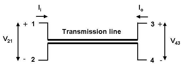
The following y-parameter equations describe the transmission line.

where,

where β is the propagation factor and l is the length of the line. After transformers, we obtain,

NODE 1

NODE 2

NODE 3

NODE 4

There is one small problem with the above formulation for transformers and transmission lines. The network formulation of SOLVE requires that there be one node connected to one earth yet both transmission lines and transformers have floating inputs and outputs. Only the input or the output can be directly connected to earth. Moreover one often wants to float the output. The solution is to connect a large value resistor from the output earth to the earth, where by large we mean much larger than the magnitude of the impedances in the system.

EXAMPLES

To put these ideas into practice and to give an example of how to treat the transistor, we look at a simple example for the transformer and a more complex example for transmission lines.

(1) Consider the following 1:1 transformer.



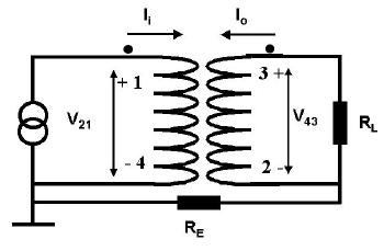
The following matlab program can be run with solve.m to analyse the circuit for Nvals = 300 frequencies from 10 to 1000 MHz. Note the use of R_E = 1 MΩ resistor to connect the primary and secondary earths together. There are N = 4 circuit nodes and only N by N-1 y's are required (i.e. we ignore the direction from every node to ground).

clear all %Need to provide Nvals... the number of frequency points
Nvals = 300;
N = 4;
y = zeros(N,N-1,Nvals);

frequency = linspace(1.e7,1.e9,Nvals);
omega = 2*pi*frequency;
RL = 50.;
RE = 1.e6;
cc = 3.e8;
L = 1.e-6;
M = 9.99e-7;
beta = 2*pi*frequency/cc;
yi = (j*omega*L)./(omega.^2*(M^2 - L^2));
yT = -(j*omega*M)./(omega.^2*(M^2 - L^2));
y(4,1,:) = yi;
y(3,1,:) = -yT;
y(2,1,:) = yT;

y(3,2,:) = yi + 1/RL;;
y(4,2,:) = -yT + 1/RE;
y(1,2,:) = yT;

y(2,3,:) = yi + 1/RL;
y(1,3,:) = -yT;
y(4,3,:) = yT;

The main terms of importance are the y's, with the current souce connected to node 1 and the N = 4 node at ground. Looking at the definitions of the admittances for the transformer in section 4.2 above, the coefficients of the voltages give the admittance values. In the case of y(3,2,:) and y(2,3,:), there is also the load resistance. In the case of y(4,2,:) there is the secondary earth resistor.

(2) The following 4:9 Guanella balun looks pretty scary from the algebra point of view. The balun is OK for about a 1:2 match independent of frequency. This is because it obeys the phase lag principle from input to output. The aim is to find the input impedance.



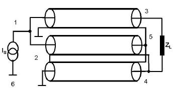
For such a balun to function correctly, it can be shown that the characteristic impedance of the transmission lines must be given by (Z_SZ_L)^1/2. Since Z_S = 50Ω and Z_L = 9/4Z_S = 112.5 Ω , Z_o = 75Ω .

The following MATLAB code does the job.

clear all
%Need to provide Nvals... the number of frequency points
Nvals = 300;
N = 6;
y = zeros(N,N-1,Nvals);
frequency = linspace(1.e7,1.e9,Nvals);
omega = 2*pi*frequency;
ZL = 112.5;
RE = 1.e6;
cc = 3.e8;
Zo = 75.
l = 1.;
beta = 2*pi*frequency/cc;

yi = 1./(j*Zo*tan(beta*l)); yT = -1./(j*Zo*sin(beta*l));

y(6,1,:) = yi;
y(2,1,:) = yi;
y(3,1,:) = -yT;
y(4,1,:) = yT;
y(5,1,:) = yT - yT;

y(6,2,:) = yi;
y(1,2,:) = yi;

y(1,3,:) = -yT;
y(4,3,:) = 1/ZL;
y(5,3,:) = yi;
y(6,3,:) = yT;

y(1,4,:) = yT;
y(3,4,:) = 1/ZL;
y(2,4,:) = yT - yT;
y(5,4,:) = 2*yi;
y(6,4,:) = -yT + 1/RE;

y(3,5,:) = yi;
y(4,5,:) = 2*yi;
y(2,5,:) = yT - yT;
y(6,5,:) = yT - yT;
y(1,5,:) = yT - yT;