Spherical Harmonic Plotting with MATLAB®
Technical Note — 6 Aug 2015Contents
MATLAB® Code generate_spherical_harmonic.m
Note that the spherical harmonic is not normalized since we are interested in the shape and not the scaling.
function [x,y,z,yyhat,name]= generate_spherical_harmonic( degree, order, type, theta1, theta2, phi1, phi2, rho_ref, rho_scale, alpha, beta, gamma, numt, nump )
%GENERATE_SPHERICAL_HARMONIC computes a mesh for a spherical harmonic
%   degree - non-negative integer
%   order - non-negative integer between 0 and degree (these are real spherical harmonics
%   type - 0 means the cos type or real type, 1 means the sin type or image type
%   theta1/theta2 start/end theta of patch (theta2<theta1 is permitted)
%   phi1/phi2 start/end phi of patch (phi2<phi1 is permitted)
%   rho_ref - radius of reference sphere; try 0.0 or 1.0
%   rho_scale - multiplier for normalised (max(abs())=1) spherical harmonic; try 1.25 or 0.25
%   alpha - third rotation in radians about z-axis
%   beta - second rotation in radians about y-axis
%   gamma - first rotation in radians about z-axis
%   numt - grid size theta
%   nump - grid size phi

	% Map degree and order to valid ranges
	degree=abs(degree);
	order=min(abs(order),degree);

	% Create the standard uniform grid in both angles
	theta3=linspace(theta1*pi/180,theta2*pi/180,numt);
	phi3=linspace(phi1*pi/180,phi2*pi/180,nump);
	[theta,phi]=meshgrid(theta3,phi3);

	% Calculate the bank of Legendre functions (of all orders)
	Ylm=legendre(degree,cos(theta3));
	if degree==0
		Ylm=Ylm'; % thanks a lot matlab
	end

	% pull out the associated Legendre function of the desired order
	Ylm=Ylm(order+1,:); % row of the desired order
	yy=kron(ones(size(phi3')),Ylm); % repeat this row ready for multiplying with mesh phi term

	% construct the SH
	if type==0 % real part
		yy=yy.*cos(order*phi);
	elseif type==1 % imag part
		yy=yy.*sin(order*phi);
	end

	% normalize SH so that it has values in range [-1,+1]
	yymax=max(max(abs(yy)));
	if yymax==0 % zero function
		yyhat=zeros(size(yy));
	else
		yyhat=yy/yymax;
    end

	% map the SH value to the radial (height) value
	rho_scale=max(rho_scale,0.005); % not too small
	rhoabs=abs(rho_ref+rho_scale*yyhat);

	% Apply spherical coordinate equations
	x=rhoabs.*sin(theta).*cos(phi);
	y=rhoabs.*sin(theta).*sin(phi);
	z=rhoabs.*cos(theta);

	% rotate the mesh according to zyz Euler rotation
	R=RZRYRZdeg(alpha,beta,gamma);
	Rxyz=R*[x(:) y(:) z(:)]'; % vectorize mesh matrices
	% refill mesh matrices from vector answer Rxyz
	x(:)=Rxyz(1,:)';
	y(:)=Rxyz(2,:)';
	z(:)=Rxyz(3,:)';

	if type==0
		name=sprintf('%02u-%02u-real',degree, order);
	else
		name=sprintf('%02u-%02u-imag',degree, order);
	end
end
MATLAB® Code RZRYRZdeg.m
function [ R ] = RZRYRZdeg( alpha, beta, gamma )
%RZRYRZDEG Generates the 3x3 'zyz' matrix corresponding the Euler angles
%   arguments in deg
%   gamma is the first rotation about the z-axis
%   beta is the second rotation about the y-axis
%   alpha is the third rotation about the z-axis
	alpha=alpha*pi/180;
	beta=beta*pi/180;
	gamma=gamma*pi/180;
	Rz1=[cos(gamma) -sin(gamma) 0; sin(gamma) cos(gamma) 0; 0 0 1];
	Ry=[cos(beta) 0 sin(beta); 0 1 0; -sin(beta) 0 cos(beta)];
	Rz2=[cos(alpha) -sin(alpha) 0; sin(alpha) cos(alpha) 0; 0 0 1];
	R=Rz2*Ry*Rz1;
end
Examples
Here we demonstrate some uses of the above MATLAB® functions.
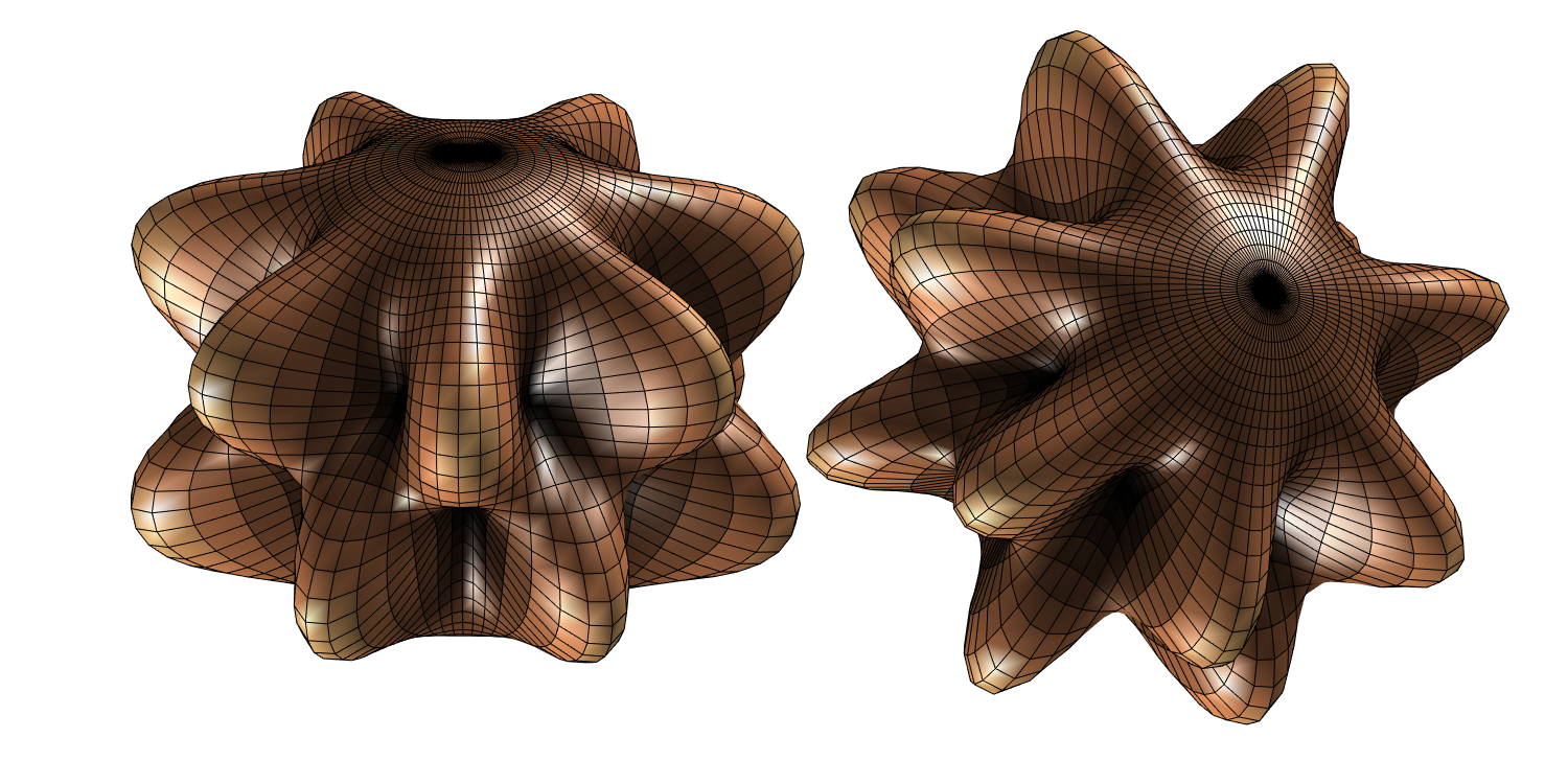
1) MATLAB® Code shex_01.m
Here we pick one spherical harmonic corresponding to and and plot it without rotation (on the left) and with a rotation through Euler angles (in degree) , and (on the right). The rotation is achieved by rotating the mesh.
function []=shex_01()
    set(gcf,'PaperUnits','inches','PaperPosition',[0 0 10 5]) %150dpi
    colormap('copper')
    subplot(1,2,1)
    plonk(0,0,0)
    subplot(1,2,2)
    plonk(270,45,0)
    saveas(gcf, 'figures/shex_01', 'png')
    shg
end

function []=plonk(alpha,beta,gamma)
    [x,y,z,f,name]= generate_spherical_harmonic(8,7,0, ...
        0,180, 0,360, 1.25, 0.5, alpha,beta,gamma, 48, 96);
    s=surf(x,y,z,f);
    set(s,'LineWidth',0.1)
    light               % add a light
    lighting gouraud    % preferred lighting for a curved surface
    lightangle(260,-45) % second fill-in light
    maxa=1.8;
    axis([-maxa maxa -maxa maxa -maxa maxa])
    axis off
    %set(s, 'edgecolor', 'none');
    camzoom(2.0)
end
Output png figure — shex_01.png
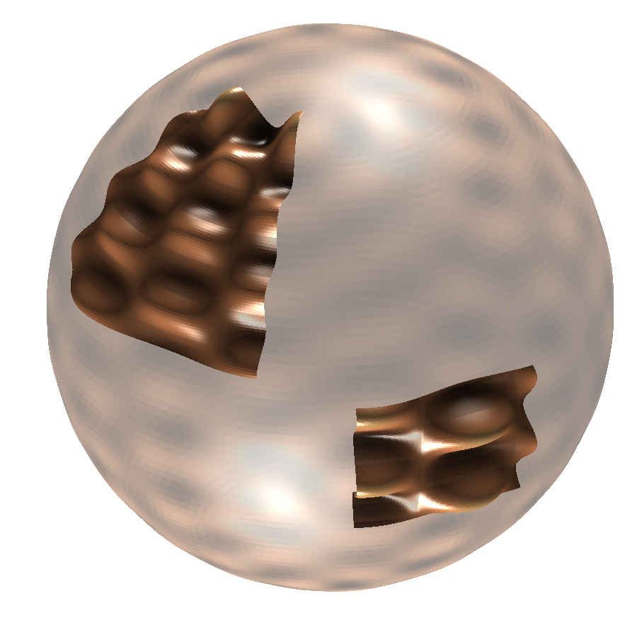
2) MATLAB® Code shex_02.m
Here we overlay patches of a spherical harmonic on a transparent sphere.
function []=shex_02()
    clf;
    colormap('copper')

    % transparent sphere
    [x,y,z,f,~]=generate_spherical_harmonic(24,8,0, 0,180, 0,360, 1.25,0.0, 0,0,0, 96,192);
    surf(x,y,z,f,'edgecolor','none','facealpha','0.3');

    % setup scene
    light               % add a light
    lightangle(260,-45) % second fill-in light
    lighting gouraud    % preferred lighting for a curved surface
    axis equal off      % set axis equal and remove axis
    view(-75,30)        % set viewpoint
    camzoom(1.7)
    hold on

    % add a patch
    [x,y,z,f,~]=generate_spherical_harmonic(24,8,0, 20,75, 120,180, 1.25,0.1, 0,0,0, 96,192);
    surf(x,y,z,f,'edgecolor','none');

    % add a patch
    [x,y,z,f,~]=generate_spherical_harmonic(24,8,0, 80,110, 200,240, 1.25,0.1, 0,0,0, 96,192);
    surf(x,y,z,f,'edgecolor','none');

    set(gcf,'PaperUnits','inches','PaperPosition',[0 0 6 6]) %150dpi
    saveas(gcf,'figures/shex_02','png')

    hold off; shg
end
Output png figure — shex_02.png
Downloads
Code Index:
[06 Sep 2016]— Latex labels with MATLAB®[21 Jul 2015]— TikZ–tikzexternalize to png[18 Jul 2015]— Spherical Harmonics LaTeX Macros[01 Aug 2015]— BibDesk Publication html Export
Sphere Index:
[06 Aug 2015]— Spherical Harmonic Plotting with MATLAB®[18 Jul 2015]— Spherical Harmonics LaTeX Macros[16 Jul 2015]— Spherical Harmonic MATLAB® Code 1
Misc Index:
[06 Aug 2017]— HLab–1[31 Jul 2015]— Outputing png from pgfornament[18 Jul 2015]— Improving Gauss-Legendre