Series RLC

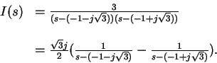
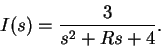
Second order circuits have two dynamic elements, e.g. the series RLC circuit of Figure 28. Let's calculate the current i(t), $t \geq 0$ .

**Figure 28:** Second-order RLC circuit.
$\begin{figure} \begin{center} \epsfig{file=images/trans2img1.eps}\end{center}\end{figure}$

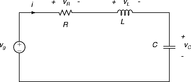
Suppose L=1 H, C=1/4 F, and R will be specified. The initial conditions are given as i(0^-) = 0 A, and v_C(0^-)=2 V. The source or input voltage is v_g(t) = 5 u(t) V.

In the s-domain, the circuit is as shown in Figure 29.

**Figure 29:** Second-order RLC circuit in s-domain.
$\begin{figure} \begin{center} \epsfig{file=images/trans2img2.eps}\end{center}\end{figure}$

Applying KVL around the loop we get

$\begin{displaymath}\frac{5}{s} = I(s) ( R + s + 4/s) + \frac{2}{s} \end{displaymath}$

and solving for current gives

$\begin{displaymath}I(s) = \frac{3}{s^2 +R s + 4} . \end{displaymath}$

(32)

The denominator polynomial gives us the characteristic equation

s² + Rs + 4 = 0 .

(33)

The roots of this equation s₁ and s₂ determine the nature of the response, and are given by

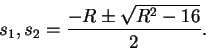
$\begin{displaymath}s_1, s_2 = \frac{-R \pm \sqrt{R^2-16}}{2} . \end{displaymath}$

(34)

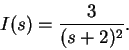
There are three cases, depending on the sign of R²-16.

Case 1. R>4 $\Omega$ , R²-16 > 0. (Overdamped.).

Let's take R=5 $\Omega$ . The two roots are

$\begin{displaymath}s_1 = -4, \ \ s_2 = -1 \end{displaymath}$

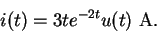
(two distinct real numbers). Therefore

s² + 5s +4 = (s+4)(s+1)

and so, from (32) we get

$\begin{displaymath}I(s) = \frac{3}{s^2 +5 s + 4} = \frac{-1}{s+4} + \frac{1}{s+1} \end{displaymath}$

using partial fractions. Transforming back we get

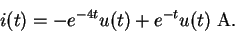
$\begin{displaymath}i(t) = -e^{-4t} u(t) + e^{-t}u(t) \ {\rm A} . \end{displaymath}$

(35)

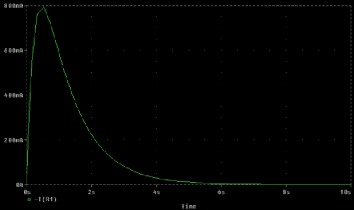
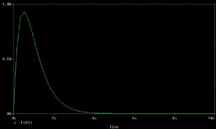
The waveform is illustrated in Figure 30.

**Figure 30:** Overdamped response.
$\begin{figure} \begin{center} \epsfig{file=images/trans2img3.eps}\end{center}\end{figure}$

Case 2. R=4 $\Omega$ , R²-16 = 0. (Critical damping.).

The two roots are

$\begin{displaymath}s_1 = -2, \ s_2 = -2 \end{displaymath}$

(two equal real numbers). From (32) we get

$\begin{displaymath}I(s) = \frac{3}{(s+2)^2} . \end{displaymath}$

Transforming back, we have

$\begin{displaymath}i(t) = 3te^{-2t} u(t) \ {\rm A} . \end{displaymath}$

(36)

The waveform is illustrated in Figure 31.

**Figure 31:** Critical response.
$\begin{figure} \begin{center} \epsfig{file=images/trans2img4.eps}\end{center}\end{figure}$

Case 3. R<4 $\Omega$ , R²-16 < 0. (Underdamped.).

Now take R=2 $\Omega$ . The roots are

$\begin{displaymath}s_1 = -1 -j \sqrt{3}, \ \ s_2 = -1 + j \sqrt{3} \end{displaymath}$

(complex conjugate pair). From (32) we get

$\begin{displaymath}\begin{array}{rl} I(s) & = \frac{3}{(s-(-1 -j \sqrt{3}))(s-(-... ...1 -j \sqrt{3})} - \frac{1}{s-(-1 + j \sqrt{3})} ) . \end{array}\end{displaymath}$

Transforming into the time domain we get

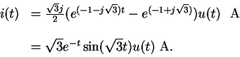
$\begin{displaymath}\begin{array}{rl} i(t) & = \frac{\sqrt{3}j}{2}( e^{(-1 -j \s... ... = \sqrt{3}e^{-t}\sin(\sqrt{3} t) u(t) \ {\rm A} . \end{array}\end{displaymath}$

(37)

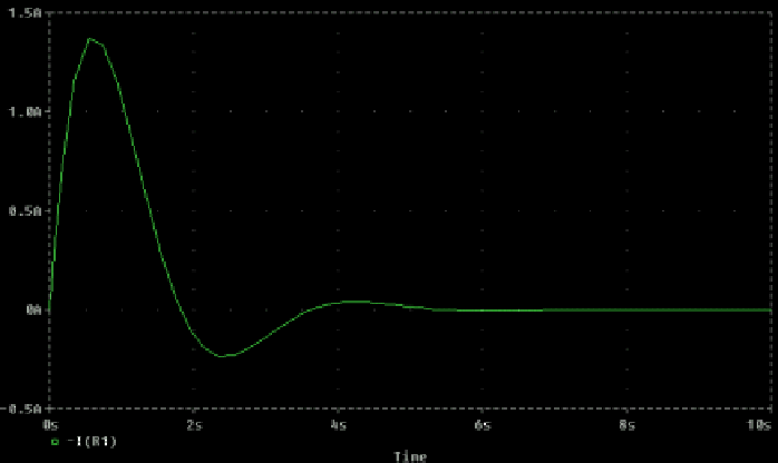
The waveform is illustrated in Figure 32.

**Figure 32:** Underdamped response.
$\begin{figure} \begin{center} \epsfig{file=images/trans2img5.eps}\end{center}\end{figure}$

[ENGN2211 Home]

ANU Engineering - ENGN2211