Author: Scott Sanner

|
Rowley-Baluja-Kanade Face Detector Author: Scott Sanner |
|
Contents
The goal of this project is to implement and analyze the Rowley-Baluja-Kanade neural net face detector as described in [2] along with some enhancements for training and recognition proposed by Sung and Poggio as described in [3]. The basic goal underlying both approaches is to train a neural network or other recognition system on a labelled database of face and non-face images. This face classifier can then be used to scan over an image resolution pyramid to determine the locations and scaling of any faces (if present) and return them to the user.
Overall, the task of face recognition can be extremely difficult given the wide variety of faces to match, the presence of facial hair, variations in lighting and shadowing, and the possibility of angular, scaling, and dimensional variances. Consequently an ideal face detector should attempt to mitigate all of these problems while achieving a high detection rate and minimizing the number of false positives. As we will see in the latter requirement, there is a tradeoff between the positive detection rate and the false positive rate and the balance between the two will need to be evaluated by the individual user and application domain.
To achieve the above goals for face detection, we use a general algorithm that is a straightforward application of data preparation, training, and image scanning. This algorithm is outlined below:
Normalize Training Data:
  - For each face and non-face image:
     - Subtract out an approximation of the shading plane
       to correct for single light source effects
     - Rescale histogram so that every image has the same
       same gray level range
  - Aggregate data into labeled data sets

Train Neural Net:
  - Until the Neural Net reaches convergence (or a decrease
    in performance on the validation set):
     - Perform gradient descent error backpropagation on
       on the neural net for the batch of all training data

Apply Face Detector to Image:
  - Build a resolution pyramid of the image by successively
    successively decreasing the image resolution at each
    level of the pyramid, stopping at some default minimum
    resolution
  - For each level of the pyramid
     - Scan over the image, applying the trained neural net
       face detector to each rectangle within the image
     - If a positive face classification is found for a
       rectangle, scale this rectangle to the size
       appropriate for the original image and add it to
       the face bounding-box set
  - Return the rectangles in the face bounding-box set
In performing face detection with a neural net, a few face-specific and non-face-specific issues arise.
In the realm of face specific issues, we do not want the background to become involved in face matching. Consequently, if person A is in two different settings we want to ensure that we perform as well as possible in detecting person A's face despite the background variation. If we were only to look at potential candidate rectangles for a face then we would receive interference from the corners which are more likely to consist of background than face pixels. Neural nets are especially susceptible to such errors since any consistencies between data in the training set (no matter how plausible a predictor of face-hood in real life) will likely be detected and exploited. Thus, as [3] suggests, it is a good idea to mask an oval within the face rectangle to prune the pixels used in training in neural net. For true face images, this usually guarantees that only pixels from the face are used as input to the neural net. For our implementation, we use the oval mask which can be seen in figure 3. The bounding rectangle for this mask is 18 x 27 pixels.
Another face specific issue is that of pose or glasses. We want to recognize a face invariant of whether a person is smiling, sad, wearing glasses, or not wearing glasses. Consequently it is important to construct a set of training data which covers a broad range of human emotions, poses, and glasses/non-glasses wearing faces. This ensures the greatest generalization when applying the face detector to faces which have not been seen before. For our dataset, we use 30 faces and their left-right flipped versions with a variety of emotions and poses as contained in the Yale Face Database [1]. It would be advantageous to have more faces and poses than this but the time limits of this project constrained the amount of time that could be devoted to photoediting (since the Yale Face Database is not in a directly usable format).
One non-face specific issue is that of lighting direction. Neural nets are especially susceptible to pixel magnitude values and the differences between images illuminated from the left or right may be enough to make them appear as two different classifications from the perspective of the neural net. Consequently, there has to be some method for correcting for unidirectional lighting effects (even if only approximate). Additionally, not all images will have the same gray level distribution or range and it is important to mitigate this as much as possible to avoid bias effects due to gray level distribution.
For our dataset, we attempt to correct for unidirectional lighting effects as suggested by [2] by fitting a single linear plane to the image. This plane can be computed efficiently through simple linear projection solving the equation [X Y 1] * C = Z (where X, Y, and Z are the vectors corresponding to their respective coordinate values, 1 is a vector of 1's to compute the constant offset, and C is a vector of three numbers defining the linear slopes in the X and Y directions and the constant offset). To compute C, we simply need to compute ([X Y O] ' * [X Y O])^-1 * [X Y O] ' * Z. These plane coefficients in C approximate the average gray level across the image under a linear constraint and thus can be used to construct a shading plane that can be subtracted out of the original image. Once the lighting direction is corrected for, the grayscale histogram can then be rescaled to span the min and maximum grayscale levels allowed by the representation.
This was done for our face (and non-face) training data and an original subset of images are shown in figure 1 below:
 Figure 1:
Initial Images.
Figure 1:
Initial Images.
From figure 1, we then approximate the shading plane as shown below. Note that the second and third images in figure 1 show heavy directional lighting effects and that the shading plane in figure 2 accurately represents these effects.
 Figure 2:
Shading Approximations.
Figure 2:
Shading Approximations.
Now, given the images in figures 1 and 2, we can subtract figure 2 from figure 1 and rescale the gray levels to the minimum and maximum range for our representation. We can then apply a mask to this image to remove background interference. This result is shown below in figure 3.
Note in the following figure that the unidirectional lighting effects present in the original second and third images (figure 1) have now been removed and that unlike figure 1, all images in figure 3 have approximately the same gray level distribution. This normalization is extremely important to proper functioning of the neural network.
 Figure 3:
Normalized and Masked Images.
Figure 3:
Normalized and Masked Images.
In addition to the face images, we also perform the same normalization on a set of non-face scenery images. Since we normalize all images during the face detection scanning process, it is important to train on normalized scenery images since the unnormalized set would be unrepresentative of those seen during training. A set of five of the 160 scenery images is shown below in figure 4. (Actually only 40 scenery images were used, but their left-right and upside-down versions were also added to the data set.)
 Figure 4:
Non-face Image Examples.
Figure 4:
Non-face Image Examples.
Once all of the training data images have been normalized they are aggregated into labelled datasets and passed on to the training phase. Additionally, the normalization process occurs once more during the actual face detection process, i.e. all images rectangles are normalized before classifying them with the neural net.
Given our mask size, we use a neural net (created and trained using Matlab's neural net toolbox) with approximately 400 input units connected directly to a corresponding pixel within the image mask, 20 hidden units, and 1 output unit used for prediction (yielding ideal training values of -0.9 for scenery and 0.9 for a face).
The neural net is trained for 500 epochs (or until error increases on an independent validation chosen separately from the training set). The sum of squares error rate on the training set (blue) and the validation set (red) are plotted below in Figure 5. Note that around epoch 50, the validation set error surpasses the training set error (as would be expected). However the validation set error never increases from a previous time step and therefore the network procedes to approximate convergence. This indicates that in some sense the training set is adequate enough to generalize to unseen instances.
 Figure
5: Training Error vs. Epochs.
Figure
5: Training Error vs. Epochs.
The final performance of the network on all of the face and non-face data is shown below in table 1. The network apparently performs much better at detecting non-faces which is probably due to the bias toward non-face training images in the data set. However, this has the advantage of yielding a lower false positive rate than if the bias had been in favor of the face images instead.
| Face Detection Rate | Non-face Detection Rate | Overall Classifcation Rate | |
| Percentage Correct | 86.7% | 98.1% | 97.7% |
| Training Set Size | 60 | 160 | 220 |
Table 1: Training Results.
Now that the neural net has been successfully trained, it can now be used for classifying candidate face rectangles passed to it from an image.
Image Scanning and Face Detection
Since we have a constant size input and constant size mask (with a bounding rectangle of 18 x 27 pixels), we need some method for scaling the image so that we can detect faces of multiple sizes. Consequently, we build an image pyramid for an image to be scanned by placing the original image at the bottom and successively scaling down the resolution between pyramid levels until some preset low resolution level has been reached. (We have found that scaling by 1.1 to 1.2 at each level yields a pyramid of adequate scaling granularity. The scaling value of 1.2 is suggested by both [2] and [3].)
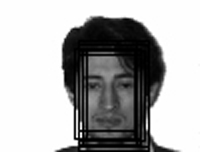
An example of an image pyramid having six levels and a scale factor of 1.2 is shown below in figure 6.
 Figure
6: Resolution Pyramid.
Figure
6: Resolution Pyramid.
Once the image pyramid is obtained, face detection is a fairly straightforward process. For each level of the image pyramid we simply want to scan over all possible rectangles. We then extract each rectangle from the image, normalize it according the procedure outlined in the data preparation section, and pass it to the neural network for classification. The neural net returns a value which can then be thresholded to determine whether that image is a face or not. It is fairly straightforward to compute the bounding box of the face for the original scaling from the image level and rectangle location. Consequently, all face bounding-boxes are stored and passed back to the calling procedure. This set of bounding boxes outlines the predicted face locations and scales in the image and can be overlayed on the image as is done below in figures 8-13.
Now that the system is defined, we can proceed to analyze it's performance. In situations where one is interested not only in the correct positive classification rate but the false negative rate as well, it can be useful to plot an ROC curve to exhibit this tradeoff.
In our case, varying the threshold of the output of the neural net yields varying performance for the correct face identification rate vs. the false positive rate. At a low threshold, we are likely to detect more faces with the caveat that we are also likely to misclassify more scenery images as faces. At a high threshold, we will likely have fewer false face detections but we will also probably fail to detect faces that were just below threshold.
Consequently, in the following table we have run our face detection system with a number of images and thresholds and tallied the correct face identification rate and the false positive rates over all images. The number for the false positive rate is the number of false positives out of all rectangles classified for the set of images (6500 in this case). One can easily see the tradeoff between correct face identification rate and false positive rate as a function of the threshold as mentioned above.
| Threshold | Correct Face ID Rate | False Positive Rate |
| 0.0 | 1.00 | 35/6500 |
| 0.1 | 1.00 | 21/6500 |
| 0.2 | 1.00 | 15/6500 |
| 0.3 | 0.857 | 7/6500 |
| 0.4 | 0.714 | 6/6500 |
| 0.5 | 0.714 | 4/6500 |
| 0.6 | 0.571 | 3/6500 |
| 0.7 | 0.429 | 1/6500 |
| 0.8 | 0.286 | 0/6500 |
| 0.9 | 0.000 | 0/6500 |
Table 2: Face Detection and False Positive Rates for Face Detector.
The data in the above table is also plotted graphically below in figure 7. This shows the correct face identification rate as a function of the false positive rate for different values of the threshold parameter (shown next to each data point ranging from 0.0 to 0.9). Here it is quite apparent that one achieves better face identification rates at the cost of increased false positive rates.
 Figure
7: ROC Plot for Face Detector.
Figure
7: ROC Plot for Face Detector.
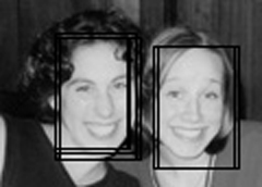
So, how does the face detector perform on actual images? Two sample runs on fairly clean images (which have not been used in training) are shown in figures 8 and 9. Here we see a number of rectangles at different scales which all pick up the faces in both pictures. Given the lack of scenery in the background, we really do not expect any false positives here, however the fact that the face is so well detected at different scales and positions is a good indicator that the neural network can generalize well (especially since it has never seen these faces before)! The threshold used in both of these images was 0.5.
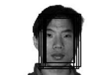 |
 |
Figures 8-9: Examples of Face Detector Application to Clean Images.
We now proceed to slightly more complex images with scenery that have not been trained on. Here there was an incidence of a number of false positives at scales much larger than those where faces were correctly detected. These levels of the image pyramid were thrown out so that we can see how the system performed at the correct range of scales (and it does work quite well here, having only one false positive in figure 11). The threshold for both of the following images was set at 0.5.
The occurrence of false positives at scales larger than the detected faces is due to the presence of high frequency features in large rectangles which are mistaken as facial features. This indicates a fwe improvements that could be made to the neural network and training set that will be discussed in the conclusion.
 |
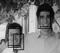 |
Figures 10-11: Examples of Face Detector Application to Complex Images.
We now proceed to a complex image shown in figures 12 and 13 with 7 faces. These images demonstrate the tradeoff between correct face identification rate and false positive rate. Figure 11 was computed with a threshold of 0.2 and figure 13 was computed with a threshold of 0.6.
It is quite apparent that for a low threshold as in figure 12, we do correctly identify all 7 faces (look closely and this will be apparent) but at the cost of an unacceptable number of false positive identifications.
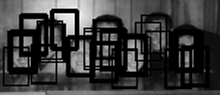 Figure
12: Example of Low Threshold.
Figure
12: Example of Low Threshold.
In figure 13, we have just the opposite happen with very few false positives but a correct positive identification of only 5 of the 7 faces (again, look closely and this will be apparent). The system misses the second face from the left and right probably due to the rotation of both of these heads.
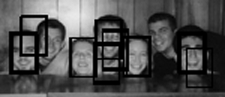 Figure
13: Example of High Threshold.
Figure
13: Example of High Threshold.
Consequently, we see that the face detection system performs fairly well with a few caveats - namely a large number of false positive identifications under thresholds required to identify all faces in an image and at resolution scales which are much larger than those where the faces are detected. This suggests some modifications to the system which will be addressed in the next section.
We will first cover the strengths of this face detection system implementation and then move onto its caveats and possible improvements to address these problems.
Perhaps one of the most important components of the face detector and in fact independent of the classification method used (e.g. neural network or eigenface projection) is the image normalization routine. Most face classification systems are highly sensitive to the gray levels in an image and in tests conducted with this system, running the face detection without normalization yielded completely unusable results. Consequently, the ability to take arbitrary images of a face with different lighting directions and gray-level histograms and project them onto a canonical lighting and gray-level distribution is extremely useful. It allows for the classification of a whole range of faces that would otherwise be completely missed. Furthermore, as outlined by the methods above, it is also fairly computationally efficient given the small size of the matrices used during normalization.
One of the other important components of this project is the wide range of emotions, poses, and lighting found in the training data set. The fact that only 30 face images and their reversed versions could yield such generalization results on the above photos is fairly impressive. This includes another important point: It is useful to have flipped and rotated versions of the images to allow for translational and rotational invariance. The data set used in this system accounted for translation invariance but as seen in the missed classifications on figure 13 due to rotational invariance, it could benefit from having slightly rotated versions of the training images (which was not done on account of time constraints).
Despite its success and aside from missed postive classifications, this system's major drawback is that it suffers from a high false positive rate on some images. This is primarily due to two issues:
1) Both [2] and [3] mentioned that their systems were initially trained on a set of randomly generated images to bias the network towards non-face classification in the lack of features to suggest a face. This was not done for this face detection system and it seems that some of the false positives are simply due to random fluctuations of the neural net on images which do not match well with either the face or non-face training data.
2) The system implemented in [2] used a novel neural net connection scheme that was modelled after the retina. That is, it had units for horizontal bars, vertical bars, and rectangles within the image. These unit connections facilitate high-level feature aggregation and are less susceptible to noise than the one-to-one correspondance between pixels and neural net inputs used in this system. Since high-frequency noise seems to be a major cause of false negatives (as in figures 10 and 11 where rectangles much larger than the faces had incorrectly matched high frequency non-face features), the noise reduction in a 'retinally-connected' neural network would seem to be extremely advantageous.
Consequently, the system yields some fairly impressive results in the tests but could likely benefit from additional enhancements as mentioned in [2] and [3]. However, given the time constraints on this project, it seems fascinating that the system can take an arbitrary image and usually with little tweaking, return a fairly accurate set of bounding boxes for faces at a number of scales (try it out!). This at the very least suggests that the basic approach used here is highly effective and could likely benefit from the improvements suggested above to increase positive detections while decreasing the rate of false positives (i.e. the ROC characteristics).
[1] Yale Face Database. Available at http://cvc.yale.edu/projects/yalefaces/yalefaces.html.
[2] H. A. Rowley, S. Baluja, and T. Kanade. "Human face detection in visual scenes." CMU-CS-95-158R, Carnegie Mellon University, November 1995. Available at http://www.ri.cmu.edu/pubs/pub_926_text.html.
[3] T. Poggio, and K.K. Sung. "Example-based learning for view-based human face detection." Proc. of the ARPA Image Understanding Workshop, II:843-850. 1994. Available at http://citeseer.nj.nec.com/poggio94examplebased.html.
The software for this project is archived in the tar-file fd.tar.gz. The README file within this archive contains instructions on how to set up and use the face detection system. It is excerpted below.
README (Bundled with Software Archive)
Student: Scott Sanner
Email:   ssanner@cs.stanford.edu
Course:  CS223B, Winter
Final Project: Rowley-Beluja-Kanade Face Detector

System Requirements
===================
Matlab 5.x with the Image Processing and Neural Net
toolboxes.

Unpacking the files
===================
Create a directory for the project and untar the tarfile
using the command 'tar -xvzf fd.tar.gz'.  This should create
a number of m-files in the current directory and a
subdirectory of images used to train the neural net.

Running the Face Detector
=========================
To build a trained, face-detection neural net, simply
run the 'facetrain' script.  The two global variables needed
from this script are 'NET' which is the trained neural net,
and 'MASK' which is the mask used to define the area inside
a rectangle which will be tested for facehood.

To run the face-detector on an image using the 'facescan'
function, simply pass 'NET', 'MASK', a double array of the
grayscale image, and a few parameters governing the
detection threshold and image scanning characteristics.
Check the 'facescan.m' file for more information on good
values for the paramters.

File Listing
============

M-Files (Main Files)
--------------------
facetrain.m     - The main neural net training script
                  which loads all required training files,
                  builds the needed data structures,
                  and trains and tests the neural net

facescan.m      - The main image face-scanning function.
                  Simply pass this function the neural
                  net, image, mask, and a few parameters
                  governing the detection threshold and
                  scanning characteristics.  See the
                  contents of this file for for good
                  default values for the parameters.

M-Files (Neural Net Utilities)
------------------------------
createnn.m       - Creates a neural net given the input,
                   hidden, and output unit characteristics.
simnn.m          - Simple formats the data for presentation
                   to the neural net.
trainnn.m        - Trains a neural net given labeled data
                   and a percentage to use for the
                   validation set (which it constructs).
classifynn.m     - Normalizes an image and returns the
                   classification value from the neural net.

M-Files (Image Utilities)
-------------------------
buildimvector.m  - Builds an image vector from a rectangular
                   image array.  Used to convert data so
                   that it can be used by the neural net
                   for training.
buildresvector.m - Builds a result vector to match the
                   image vector.
buildmask.m      - Builds a rectangulary binary mask array
                   for face images.
normalize.m      - Normalizes an image by subtracting a
                   linear lighting plane and rescaling the
                   grayscale distribution histogram.
augmentlr.m      - Augments an image set with the left-right
                   flipped versions of the images.
augmentud.m      - Augments an image set with the upside-
                   down versions of the images.

M-Files (Image Loading/Display)
-------------------------------
loadimages.m     - Loads a set of images according to the
                   given pattern set.
showimages.m     - Subplots a set of images in an image
                   array.

Image Data (Using wildcards '#')
--------------------------------
scaled/n##-x.PNG - Non-face files used for training
scaled/s##-n.PNG - Face data of normal pose for s##
scaled/s##-c.PNG - Face data of center lighting pose for s##
scaled/s##-l.PNG - Face data of left lighting pose for s##
scaled/s##-r.PNG - Face data of right lighting pose for s##
scaled/s##-g.PNG - Face data of pose with glasses for s##